ARIADNE

Motivation

Surface defect identification is an important problem in many industrial processes, and is often accomplished through automated optical inspection (AOI). In printed circuit board (PCB) manufacture, catching defects early in the production chain is extremely important; disconnected or shorted nets can be very difficult to diagnose or QA test in a final assembly. Automated optical inspection is thus widely deployed in the PCB industry, and is a topic of ongoing research in CV/ML; the latency and accuracy constraints are significant, since AOI operates as an online, interstitial part of the production line.

I am specifically interested in not just classifying, but locating defects; both methods thus focus on obtaining bounding boxes around each defect identified, and classifying those defects in an ontology useful to PCB lithographers. Go/no-go decisions on an entire board image are sufficient for immediate control of the assembly line, but data on fault location and type is useful long-term; for instance, one can produce heatmaps of fault locations, or identify specific lithomasking machines which need servicing based on fault type distribution.

Since PCB manufacturing is generally done via photomasking, our source masks form a perfect ground truth description of each of the target PCB's copper layers; this reduces the AOI problem to comparison between the "template" mask source image and a scan of the post-etching copper layer. Additionally, since circuit boards are generally extremely flat, dimensionally accurate, and formed of uniform material, the imaging environment can be heavily constrained to remove most obstacles to registration and comparison.

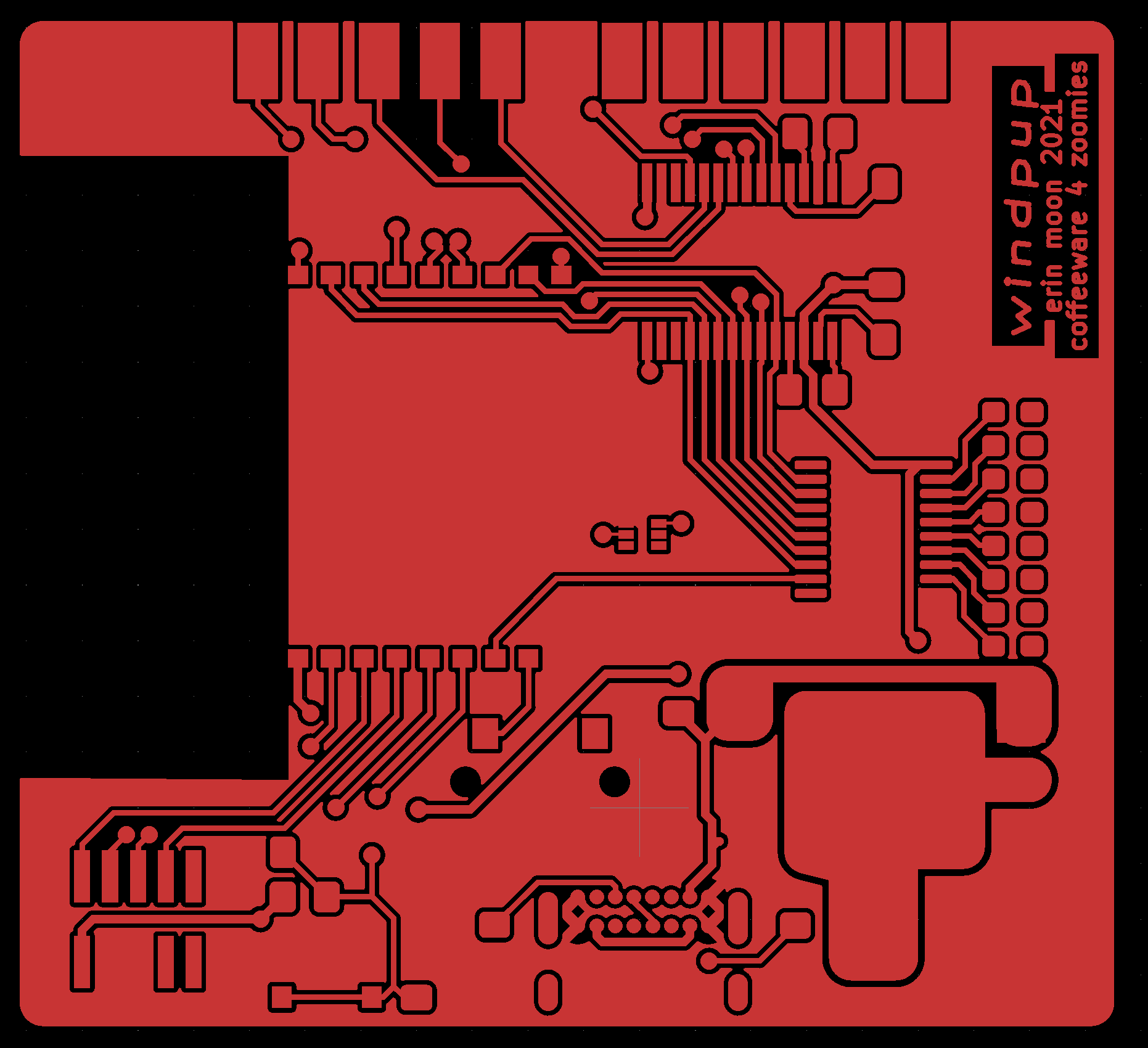
An example copper layer mask from a board design by the author; this is a `gerbview` visualization of one of the Gerber files which was sent to fab.

Given the above problem description, I chose to focus on comparison of observed copper layers with the source lithomasks. I implemented two fault detectors: a naive, morphology-based CV method and a (semi-)novel transfer learning method of my own design, and compared their performance on a real-world-like Unfortunately, board fabrication houses generally operate as clients of other companies and do not own the IP they fabricate; as such, they cannot release production AOI datasets even if they wanted to. dataset.

Dataset

There is only one dataset of note for PCB trace inspection—DeepPCB—but it is high quality, captured via linear CCD scanning, and pre-binarized; this is similar to how boards are actually imaged in factories. Since this dataset is high quality, and trace inspection is a relatively well-constrained problem, I chose to use it as the core of my project work.

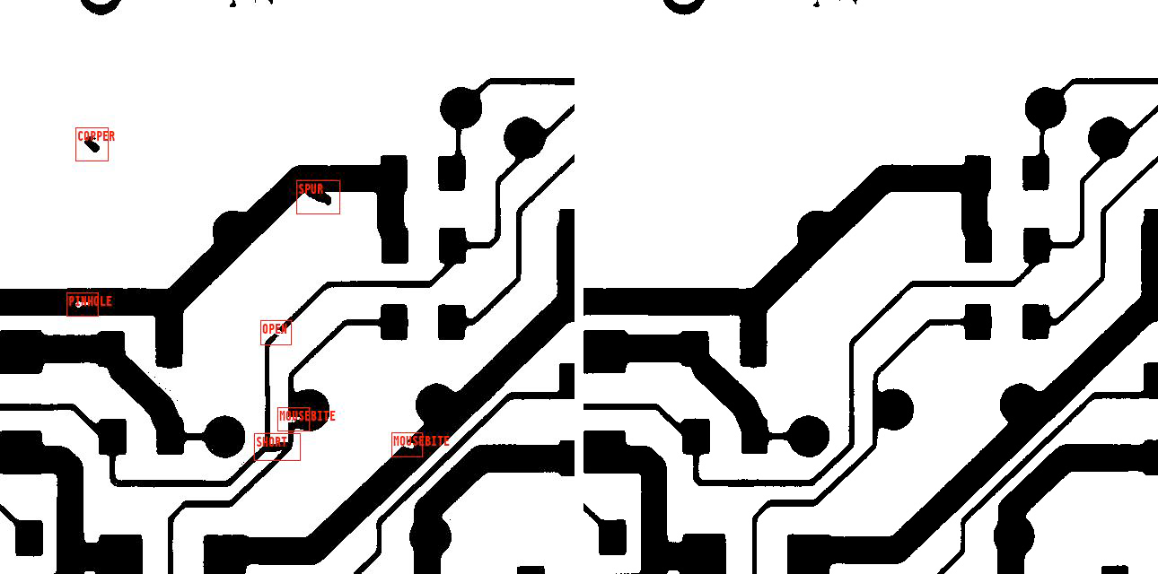
The dataset contains 1500 pairs of (reference image, observed image potentially containing defects); defects are annotated with a bounding box and type. The defect classes enumerated by the authors are:

OPEN: a full cut (region of missing copper) through a board trace
SHORT: stray copper which electrically misconnects two board traces
MOUSEBITE: a partial cut through a trace; the net is still connected, but tapers inappropriately at the defect
SPUR: a protrusion from a copper region which does not result in a short
COPPER: a misdeposition of copper disconnected from any nets, often a speck or a blob
PINHOLE: a spot of missing copper within a larger copper region

The annotations are provided in an ad-hoc text form, with one bbox and defect type per line. I wrote a small adapter in my Python codebase to parse these forms and crawl the whole dataset, providing it through a simple iterator interface that I can either peruse manually for the CV method or shim to a torch.utils.data.Dataset for the DNN object detector.

Methodology

Classical CV

I am lucky to use a dataset which provides well-aligned pairs of clean binarized images as a starting point; due to low noise tolerance in traditional CV AOI methods, physically conditioning the imaging environment is extremely important, and that work has already been done for me. As such, I designed and implemented All image processing is performed via scikit-image. a naive procedure to identify defect regions, given the pair of a reference template and observed board:

XOR the ground truth and observed images to produce a difference mask
Perform binary opening on this mask to eliminate spidery structures.
Perform binary opening on this mask to regenerate original boundaries.
Remove small holes.
Remove any straggler small connected objects.
Label the image via connected component analysis.

We then proceed to classify the labeled image. For each labeled defect, I

Discard defects with under a threshold number of pixels. Likely redundant given the above steps.
Compute the contour of the defect, via marching squares.
Compute white fractions (effectively, binary histogram) for the inner pixels and rim pixels of the defect in both the template and observed image.

A defect identified from the xor defect map, and histograms of its body and edge pixel value distribution in the observed image.

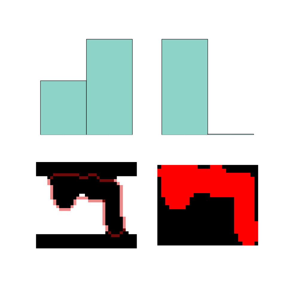
This produces a feature vector; instead of manually picking heuristic thresholds, I train a one-versus-one SVM classifier Via scikit-learn's SVC. with a radial basis kernel on the defect region features. Intuitively, by computing the pixel distribution of an identified defect in both the template and observed image, we can determine whether the region contains erroneous copper, or is an erroneous void.

If featurization fails (more than one continuous contour), or a ground truth bbox does not overlap an identified bbox during training, the object is discarded. Likewise, when predicting, if a defect cannot be featurized, it is considered a classification error.

Pairwise (Faster) R-CNNs: bifurcating the backbone

I chose to pose defect identification as an object detection problem: given two images of a copper layer, report bboxes and classes for all differences. Faster R-CNN Faster R-CNN: Towards Real-Time Object Detection with Region Proposal Networks, S. Ren et al, 2015. provided the underlying model architecture; I used a pretrained ResNet50 CNN backbone, extracting feature maps from inner layers and passing them through a feature pyramid network See Feature Pyramid Networks for Object Detection, Lin et al, 2017. . I unfroze layer2–layer4 to fine-tune the backbone.

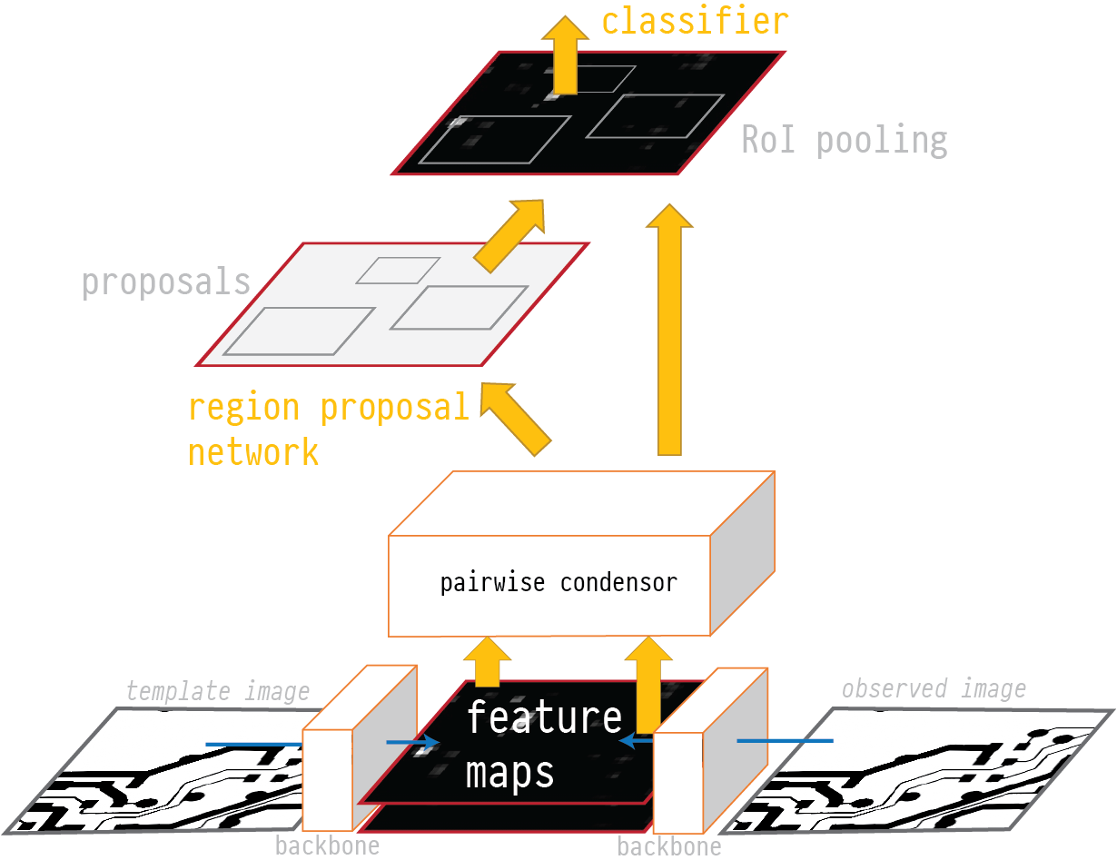
At a high level, Faster R-CNN operates by sliding a fully-convolutional attention module, the region proposal network, over the input feature maps; this produces proposed anchors at each position of the RPN's sliding window. This is used to guide RoI pooling in an underlying jointly trained Fast R-CNN network, which produces final scores and classes.

R-CNNs are designed to take a single feature map, extracted from a single image, as input; I thus had to extend the architecture to support the problem of pairwise comparison. To detect objects corresponding to differences between two images, I run the backbone over both images to featurize them, then pass these maps through a unit I term the "pairwise condensor" to reduce them to a single feature map of differences. In my initial implementation, this condensor is simply a subtraction between the feature maps, but it would be possible to use any trainable module which takes two feature maps as input and produces one as output.

The **Pairwise Faster R-CNN** (PFaR-CNN) architecture.

Results

I implemented the described pairwise R-CNN architecture in PyTorch, extending the existing torchvision systems for R-CNNs and object detectors. The model was trained for 28 epochs, across a 1000-pair subset of the 1500-pair dataset; I augmented training data with vertical and horizontal flips (p=.5). To evaluate performance, I used the pycocotools implementation of the mAP (mean average precision) and mAR (mean average recall) object detection metrics.

For the traditional CV implementation, I fit the SVM with the same size of train/test split and evaluated mAP/mAR. While evaluating both methods, I also captured average inference runtime; PFaR-CNN performance was evaluated on an Nvidia A100 (A100-SXM4-40GB), while CV performance was measured on an Apple M1 Max (64GiB RAM, MacBookPro18,4). Note the inclusion of another naive CV model S. H Indera Putera and Z. Ibrahim, "Printed circuit board defect detection using mathematical morphology and matlab image processing tools," cited in Online PCB Defect Detector on a New PCB Defect Dataset, Tang et al, 2019 , since, as discussed in the conclusions, mine is incredibly underpowered.

Model performance.
	mAP			mAR
model	IoU=0.15	IoU=0.50	IoU=0.75	IoU=0.15	IoU=0.50	IoU=0.75	inferences/sec
PFaR-CNN	.995	.990	.920	.999	.997	.950	18.69
Naive CV	.230	.0002	—	.402	.0042	—	31.95
CV (Putera and Ibrahim, via Tang et al)	—	.893	—	—	—	—	78

Observations and future work

My CV implementation is pitiful and likely buggy; I poured most of the project time into the R-CNN defect detector, and we did not cover very much morphological processing in this class. It is completely unfair to compare against it; this is why I included the Putera and Ibrahim CV performance. It could absolutely be improved, as evidenced by this other image-processing-based model; I would probably start by exploiting connected component analyses more extensively to classify defects. Additionally, my method has another disadvantage when performing COCO-style IoU/mAP evaluations: the DeepPCB dataset significantly oversizes its bboxes, whereas my model tends to predict the tightest possible bounding box, artificially deflating IoU even if the predicted bbox is completely contained within the ground truth. This means that I have to decrease the IoU threshold to comically low values, as seen in Table 1, for the COCO methodology to match ground truth with prediction whatsoever. My

The R-CNN has acceptable, but unimpressive performance, both in its predictions and its runtime. The condensor's extreme simplicity and linearity are a potential issue; it would be reasonable to explore replacing it with other modules that could learn a more sophisticated representation of difference in feature pyramids. Additionally, this is not a truly novel approach; it is very similar to the method evaluated by Tang et al. Online PCB Defect Detector on a New PCB Defect Dataset, Tang et al, 2019 . Finally, the loss optimized during training was simply the sum of the objectness loss, box regression loss, and classifier loss; it would be prudent to adjust this objective to maximize recall, since missing a defect is significantly detrimental to a production run of PCBs.

In general, this type of "spot the difference" problem—given two input images, classify the differences—is, as far as I can tell, rarely studied in CV/ML, which is somewhat surprising! Producing a semantic diff of images seems useful in other applications, and this work offers many extension points to work towards that goal. Again, the PFaR-CNN approach is not novel; the main contribution my work offers is pragmatic. By releasing code, and putting in a significant amount of effort to extend existing object detection mechanisms used in torchvision, this project establishes a basis for further work in difference detection via deep CNNs.